Statistical Hypothesis Testing with Parametric Tests

Many scientific fields require methods for making statistical inferences with the data that was generated during reserach. A cornerstone of statistical inference is hypothesis testing, which is a method used in many research scenarios. In this article, we will look into the key elements and the general procedure to conduct a hypothesis test according to modern standards. Additionally, we will examine two selected hypothesis testing methods in detail and.

The Hypothesis Testing Framework

The field of statistics can be separated into two general paradigms regarding their applications. First, there are descriptive statistics, which are applied to summarize or describe features of obtained data. On the contrary, there are inferential statistics for drawing conclusions about a population with the help of data obtained from samples. Many issues occurring in inferential statistics can be classified into one of three categories, estimation, confidence sets, or hypothesis testing. The latter of the three categories, hypothesis testing, has a broad range of applications and is used in practically all scientific fields.

Before we look at the hypothesis testing procedure, the meaning of hypothesis testing and the general approach must be defined. As already explained, hypothesis testing is a method of statistical inference, with the approach to hypothesis testing varying if we look at different paradigms of statistical inference. The article is focused on the null hypothesis significance testing framework, which resulted from combining the work of Fisher and Pearson- Neyman into a single approach. Going forward, when the term hypothesis testing is mentioned, it is in the context of the null hypothesis significance testing framework.

Null Hypothesis and Alternative Hypothesis

The process of hypothesis testing is, at its core, a decision problem and very similar to the scientific method in general. The decision is between two hypotheses that make assumptions about the parameters of a population. First, there is the null hypothesis, which is denoted by \(H_{0}\). The null hypothesis is assumed to be true until it is proven false. On the other hand, there is the alternative hypothesis, denoted by \(H_{1}\). The alternative hypothesis is declared true if the null hypothesis is disproven. Given that researchers often use hypothesis testing to prove an effect of some sort, most of the time, the null hypothesis claims that there is no effect. In contrast, the alternative hypothesis claims that an effect exists.

So in summary, first the status quo is observed, followed by the setting up of a theory, which is then tested and compared against the test results. After the evaluation of the test results, the hypothesis is then rejected or further examined.

Parametric and Non-Parametric Tests

After defining the null and alternative hypotheses, we can further specify the hypothesis testing framework. It is crucial to make a distinction between the two types of hypothesis testing. The first type of test is the parametric test, which is based on the assumption that the population from which the sample data for the test is drawn follows a particular distribution with corresponding parameters. Most of the time, there is an assumption of a normal distribution. Contrary to parametric tests, non-parametric tests are conducted without making any assumptions about the population’s distribution. The type of test to conduct must be chosen according to the tested hypothesis and the available sample data. Going forward, we will focus on parametric hypothesis tests.

Test Statistics

To conduct a hypothesis test, a test statistic is necessary. The test statistic acts as the foundation on which the decision to reject the null hypothesis is made. A test statistic is thus a function used to evaluate the sample data. The resulting value of the test statistic is a single number representing all the sample data. There are various hypothesis tests, with each test employing its own specific test statistic, for example, the t-test uses the t-statistic, while the chi-squared test uses the chi-squared statistic. Like the choice of test type in general, the selection of a specific test statistic depends on the nature of the research question and the type of data being analyzed.

Significance Level

The next necessity for a successful hypothesis test are the rules for interpreting the values derived from the test statistic. To identify when a null hypothesis has to be rejected, a significance level must be determined. The significance level denoted by \(\alpha\) is thereby the limit of how unlikely a computed value of a test statistic must be before the null hypothesis is rejected. The significance level also defines a range of resulting test statistic values, which leads to a rejection of the null hypothesis. This range of values is called the rejection region. The value for the significance level must be defined before conducting a hypothesis test and can be chosen arbitrarily, although the value should not be greater than 10 percent.

Population and Sample Distribution

Like already mentioned, most parametric tests assume a normally distributed population. If the population distribution is normal, then the sample data’s distribution is also normal. Additionally, suppose the population is assumed to be non-normally distributed. According to the central limit theorem, the sampling distribution can nonetheless be assumed to be normal for a sufficiently large sample size. In this case, the sampling distribution approaches a normal distribution when the sample size increases. If not stated otherwise for a specific testing method, a sample size of 30 is large enough to assume the sampling distribution is approximately normal.

Two-Sided and One-Sided Hypothesis Tests

After looking into the sample distribution’s necessary criteria, we can now further define the types of hypothesis tests. First, we denote \(\theta\) as a population parameter and \(\theta_{0}\) as a known value. Following, we denote the null hypothesis as \(H_{0}:\theta = \theta_{0}\). The first type of test is called a two-tailed test, with \(H_{1}:\theta \neq \theta_{0}\) as the alternative hypothesis. For the second type of hypothesis test, we have the one-tailed test with either \(H_{1}:\theta > \theta_{0}\) or \(H_{1}:\theta < \theta_{0}\) as alternative hypotheses.

The hypothesis tests are thereby called tailed tests because the rejection region is located in the tail regions of the sampling distribution curve. Resulting from their respective hypothesis definitions, the two-tailed test has a rejection region in both tails each, and the one-tailed test has a rejection region in either the left tail or the right tail. Consequently, we speak of a left-tailed test or a right-tailed test.

Testing Considerations

As already explained, the type of hypothesis test is dependent on the hypothesis, and the proposed hypothesis depends on the research scenario. In a scientific setting, it is often sufficient to determine if there is any effect at all. Consequently, the two-tailed test is the most prominently used test because positive and negative effects can be tested. The consensus is to use a two-tailed test if there is no reason to use a one-tailed test. Although the one-tailed test can outperform a two-tailed test, it should only be chosen for proving an effect that can exclusively be positive or negative.

Additionally, there is the possibility that the research only cares about either a positive or negative effect. From an ethical standpoint, like for the significance value, it is essential to choose which kind of test to take before the sample data is inspected because the rejection region’s location can influence if a null hypothesis is rejected.

Interpretation of Testing Results

Considering all the previous points, we now have all the essential elements of a statistical hypothesis test. Given that the population can be assumed to be normally distributed or the central limit theorem can be employed, a hypothesis test’s overall process is as follows: The first step is to define the two hypotheses H0 and H1 according to the research question, which results in a two-tailed or one-tailed test. Second, a significance level is chosen, and the rejection region’s location concerning the test tails is determined. Following, the result is computed with the sample data and the test statistic. The next step after obtaining our computed value is the correct interpretation of the results. From this point on, there are two general possibilities for interpretation. First, the critical-value approach and second, test interpretation with a p-value.

Critical-Value Approach

For the critical-value approach, we interpret the computed value with the help of a table. The computed value is thereby compared to the table’s values, resulting in a decision to reject or fail to reject the null hypothesis. Which table to choose depends on the distribution of the respective hypothesis test, for example, the normal distribution table, the t-distribution table, or the F-distribution table. How to correctly interpret the test results with the respective table depends on the employed hypothesis testing method and the structure of the table itself.

The p-Value

The second method for interpreting test results is the p-value approach. The p-value, also called the attained significance level, is used to express exactly how strong or weak the rejection of the null hypothesis is. It is the probability of observing the test statistic’s calculated value under the assumption that the null hypothesis is true. A smaller p-value indicates strong evidence, and a bigger p-value indicates weak evidence against the null hypothesis.

The p-value is thereby obtained from the computed value of the test statistic. It can either be calculated with statistical software or chosen from a table. With the acquired p-value, decisions regarding the rejection of the null hypothesis can be made by comparing it to the desired significance level. If the obtained p-value is smaller than the predefined significance level, the null hypothesis is rejected.

Criticism of the p-Value Approach

I already mentioned that the null hypothesis significance testing framework combines two different paradigms into a single framework. In particular, the p-value approach combines the usage of a null and alternative hypothesis, which stems from Pearson and Neyman and the concept of the p-value from Fisher, into a single procedure. The controversy around this combination stems from the fact that the original concept of Fisher’s p-value was only a probability of observing an outcome as weird as the hypothesis test’s outcome.

There was also no prerequisite to interpret the p-value under the assumption that the null hypothesis is true because there was no second hypothesis in Fisher’s testing procedure. According to various sources, although the combination of the two paradigms is the most practiced form of hypothesis testing in current scientific research, the p-value is also one of the most misinterpreted and controversial concepts.

t-Test for Two Dependent Samples

The first of the two hypothesis tests examined in detail is the t-test for two dependent samples, which is also called the paired t-test. The characteristic of dependent samples is that every sample has a dependent second sample, and vice versa. The test is based on the t-distribution and examines the hypothesis that two dependent samplings represent two populations with different means.

An example of a paired t-test would be to test random samples of people, administer a treatment, and then perform another test. For this example, the t-test evaluates if the difference between the two sampling means is statistically significant, or, in other words, if the treatment had an effect.

Prerequisites and Assumptions

First of all, a paired t-test is conducted with interval/ratio data. Interval/ratio data has the important characteristic that it can be processed mathematically. Examples of interval or ratio data are population size, age, median income, or average times. Another prerequisite is that the samples are selected randomly and that the population from which the sampling is drawn follows a normal distribution. If the population distribution is unknown, the sampling should have a size of at least 30 to assume a normal distribution according to the central limit theorem.

Another critical assumption for the paired t-test is that both samplings’ population variances are equal. This characteristic, called homogeneity of variance, is essential with regard to the accuracy of the paired t-test. The homogeneity of variance is also a critical prerequisite to guaranteeing the reliability of other parametric tests and can be evaluated with various tests, for example, Cochran’s G test.

Testing Procedure

To start the paired t-test, like in every other hypothesis test, the null hypothesis \(H_{0}\) and the alternative hypothesis \(H_{1}\) must be defined correctly. As already explained, a hypothesis test can be one-tailed or two-tailed, depending on the established hypotheses. Given that the paired t-test is concerned with means, the null hypothesis is denoted as \(H_{0}: \mu_{1} = \mu_{2}\). For a two-tailed test, we have \(H_{1}: \mu_{1} \neq \mu_{2}\) and for a one-tailed test, we have \(H_{1}: \mu_{1} > \mu_{2}\) or \(H_{1}: \mu_{1} < \mu_{2}\) as alternative hypotheses. After defining the hypotheses, the significance level must be chosen. As already explained, for ethical reasons, this must happen before the sample data is inspected.

For computing the actual values of the test, the direct-difference method is employed. For our test data, given that we have \(n\) different test subjects, we get \(2*n\) different data entries in our sample data. The \(2*n\) data entries of the sample data are split into two dependent datasets, \(X_{1}\) and \(X_{2}\), representing, for example, a pre-test score and a post-test score of the \(n\) subjects. Additionally, each of the two dependent data points in \(X_{1}\) and \(X_{2}\) yields a difference \(D\) by subtracting \(X_{2}\) from \(X_{1}\).

Following, we sum all the differences \(D\) to \(\Sigma D\) and additionally the sum of the squares of all differences to \(\Sigma D^{2}\). The next step is to calculate the mean of the differences \(\bar{D}\) and the estimated population standard deviation of the differences \(\tilde{s}_{D}\) with

\[\bar{D}=\frac{\Sigma D}{n} \quad \quad \tilde{s}_{D}=\sqrt{\frac{\Sigma D^{2}-\frac{(\Sigma D)^{2}}{n}}{n-1}}\]

With the help of \(\tilde{s}_{D}\), the standard error of the mean difference \(s_{\bar{D}}\) can be calculated, which in turn is used to compute the t-value with the test statistic for the paired t-test and \(\bar{D}\)

\[s_{\bar{D}}=\frac{\tilde{s}_{D}}{\sqrt{n}} \quad \quad t=\frac{\bar{D}}{s_{\bar{D}}}\]

Test Intepretation

From this point on, there are two possible methods for interpreting the results of the test. The first method is the critical value approach, where the computed value \(t\) is compared to the table of Student’s t distribution, which can be found here. To correctly use the table, we need an additional parameter, the degrees of freedom, which is calculated with the formula \(df = n-1\), with \(n\) being the number of test subjects.

To evaluate the computed value with the help of the table, we first search for the row corresponding to the degrees of freedom. The column is then chosen according to the type of test (one- or two-tailed) and the significance level. The resulting cross-section is the value against which our computed value is compared. Depending on our hypothesis, there are three possible conclusions, for \(H_{0}: \mu_{1} = \mu_{2}\) the null hypothesis is rejected if the computed absolute value is equal or greater than the resulting table value; for \(H_{1}: \mu_{1} > \mu_{2}\) the null hypothesis is rejected when the computed value is positive and equal or greater than the table value; and for \(H_{1}: \mu_{1} < \mu_{2}\) the null hypothesis is rejected if the computed value is negative and the computed absolute value is equal or greater than the table value.

For the p-value approach, we choose the p-value from the t-table. First, we search for the row corresponding to the degrees of freedom for our test. Then there are two possibilities for choosing the p-value. First, if the test’s computed value is equal to the table value, depending on whether the test is one-tailed or two-tailed, the corresponding significance level is chosen from one of the first two rows on the table. Alternatively, suppose we cannot find the exact t-value in the table. In that case, the p-value can be chosen by locating the nearest bigger and smaller table values for the computed critical value and their significance levels and approximately locating the p-value between the two obtained significance levels. The resulting p-value is then compared against the significance level \(\alpha\) chosen at the beginning of the test, and if the p-value is smaller than \(\alpha\), the null hypothesis is rejected.

Single-Factor Within Subjects ANOVA

The second of the presented hypothesis testing methods is called the single-factor within-subjects analysis of variance, which is, going forward, abbreviated to SFWS-ANOVA. The SFWS-ANOVA, like the paired t-test, works on dependent samples and population means, but in contrast to the t-test, the SFWS-ANOVA can evaluate more than only two dependent samplings. In essence, the SFWS-ANOVA is used to test the hypothesis that in a set of \(k\) dependent samples with \(k \geq 2\) at least two samplings represent populations with different means.

If the test result is statistically significant, it can be concluded that at least two of the \(k\) samples belong to populations with different means. The computation of the SFWS-ANOVA’s test statistic is based on the F-distribution. An example of a SFWS-ANOVA test scenario would be a study about different treatments where the same \(n\) subjects get \(k\) different treatments, which are then compared.

Prerequisites and Assumptions

Like the paired t-test, the SFWS-ANOVA is conducted with interval/ratio data. Additionally, it is assumed that the population follows a normal distribution and that the samples are chosen randomly. The last prerequisite is called the sphericity assumption and is the SFWS-ANOVA’s equivalent to the paired t-test’s homogeneity of variance assumption. The sphericity assumption can be evaluated with Mauchly’s sphericity test. It is important to note that if the number of samples \(k\) equals two, the paired t-test and the SFWS-ANOVA yield the same results, therefore going forward, we assume that the SFWS-ANOVA is only employed for \(k \geq 3\).

Testing Procedure

As always, the test starts with the definition of \(H_{0}\) and \(H_{1}\). The null hypothesis is thereby defined as \(H_{0}: \mu_{1} = \mu_{2} = \mu_{3}\), under the prerequisite that \(k = 3\). For different \(k\) the null hypothesis must be altered accordingly. The alternative hypothesis is defined as \(H_{1}\) Not \(H_{0}\), which means that at least two of the \(k\) population means differ from each other. This notation is used because \(H_{1}: \mu_{1} \neq \mu_{2} \neq \mu_{3}\) would imply that all three means must differ from each other. Now, before inspecting the sample data, like for every hypothesis test, a significance level must be determined.

For the actual test data, given that we have $n$ subjects and $k$ samplings, we get $n*k$ dependent samples, which are split into $X_{1},…,X_{k}$ different datasets. Thereby, each $X_{k}$ represents the sample data of one of the $k$ samplings. To further process the data, for each of the subjects $k$ samplings, the sum of the scores $\Sigma S$ is calculated. In addition $\Sigma X_{T}$, which is the sum of all the $n*k$ sample scores and $\Sigma X^{2}_{T}$, which is the sum of all squared scores is computed. Going forward, the total sum of squares $S S_{T}$ and the between-conditions sum of squares $S S_{B C}$ are calculated with

\[S S_{T}=\Sigma X_{T}^{2}-\frac{\left(\Sigma X_{T}\right)^{2}}{n*k} \quad S S_{B C}=\sum_{j=1}^{k}\left[\frac{\left(\Sigma X_{j}\right)^{2}}{n}\right]-\frac{\left(\Sigma X_{T}\right)^{2}}{n*k}\]

with $\Sigma X_{j}$ denoting the sum of the $n$ samples in the $j^{th}$ sampling. With the next equation the between-subjects sum of squares $S S_{B S}$ is calculated

\[S S_{B S}=\sum_{i=1}^{n}\left[\frac{\left(\Sigma S_{i}\right)^{2}}{k}\right]-\frac{\left(\Sigma X_{T}\right)^{2}}{n*k}\]

The residual sum of squares $S S_{\mathrm{res}}$ is calculated with the help of the previous three parameters, therefore $S S_{\mathrm{res}}=S S_{T}-S S_{B C}-S S_{B S}$. Additionally the between-conditions degrees of freedom $d f_{B C}$ is calculated with $d f_{B C}=k-1$ and the residual degrees of freedom $d f_{\mathrm{res}}$ with $d f_{\mathrm{res}}=(n-1)(k-1)$. With these parameters we compute the mean square between-conditions $M S_{B C}$ and the mean square residual $M S_{\mathrm{res}}$

\[M S_{B C}=\frac{S S_{B C}}{d f_{B C}} \quad M S_{\mathrm{res}}=\frac{S S_{\mathrm{res}}}{d f_{\mathrm{res}}}\]

The last step is to calculate the F-ratio, which is the test statistic for the SFWS-ANOVA.

\[F=\frac{M S_{B C}}{M S_{\mathrm{res}}}\]

Test Interpretation

Like for the paired t-test, there is the possibility to interpret the computed value with the critical-value approach or to obtain the p-value either from a table or with computation and compare it against the chosen significance level. For the critical-value approach, the computed value is compared to one of the F-distribution tables, which can be found here. The tables are used by selecting the right table corresponding to the chosen significance level and then searching for the value in the cross-section of the calculated degrees of freedom.

For the SFWS-ANOVA, the column in the F-table, which is called the degree of freedom for the numerator, corresponds to $df_{BC}$ and the row, called the degree of freedom for the denominator, corresponds to $d f_{\mathrm{res}}$. If the computed value is equal to or greater than the table critical value, the null hypothesis is rejected, and there is the conclusion that there are at least two populations with significantly different means. It is important to note that the linked F-tables are only supposed to be used for evaluating a non-directional alternative hypothesis.

To obtain the p-value, we search for the computed value independent of the table’s specified significance level. Like for the critical value, the correct row and column correspond to the numerator and denominator. If the computed value is identical to one of the table’s values, the p-value is equal to this specific table’s significance level. If the computed value is not in the table, like for the paired t-test, we choose the nearest smaller and bigger values across the tables. The actual p-value then lies between the two significance levels of the table with the next smaller value and the table with the next bigger value. Alternatively, the exact p-value can be calculated with the help of statistical software. If the obtained p-value is smaller than the predefined significance level, the null hypothesis is rejected.

Experiment – Blood Pressure Treatment

For better comprehension, we will now look at a practical application in the form of a fictive testing scenario for a blood pressure medication. To test if the medication has any effect at all, a paired t-test on 10 subjects is employed.

Hypotheses and Significance Level

Like for every hypothesis test, first the hypotheses and the significance level are defined. For the null hypothesis, I choose $H_{0} : \mu_{1} = \mu_{2}$ and for the alternative hypothesis, $H_{1} : \mu_{1} \neq \mu_{2}$, which in turn results in a two-tailed test. The significance level is chosen as $\alpha = 0.05$.

Sampling and Sample Preparation

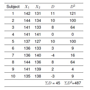
To generate the sample data, we use the Numpy library for Python, with the sample data consisting of 2 x 10 samples randomly drawn from two different normal populations. The first sample set was generated with a mean of $\mu = 140$ and a standard deviation $\sigma=5$ and the second sampling with $\mu=135$ and $\sigma=5$ to simulate a reduction of the mean systolic blood pressure of the subjects.

With this, the conditions for a normally distributed population and randomly selected samples are fulfilled. Additionally, given that $\sigma_{1} = \sigma_{2}$ and in turn $\sigma^{2}_{1} = \sigma^{2}_{2}$, the condition for homogeneity of variance is also fulfilled. Additionally the values for the differences $D$ and $D^{2}$ and the sums of the differences $\Sigma D$ and $\Sigma D^{2}$ were computed from the generated sample data. The following table features the sample data and the respective parameters.

Computation of the Test Statistic

Going forward the mean of the differences $\bar{D}$ is calculated with

\[\bar{D}=\frac{\Sigma D}{n} = \frac{45}{10} = 4.5\]

and the estimated population standard deviation of the differences $\tilde{s}_{D}$ with

\[\tilde{s}_{D}=\sqrt{\frac{\Sigma D^{2}-\frac{(\Sigma D)^{2}}{n}}{n-1}} = \sqrt{\frac{487 -\frac{(45)^{2}}{10}}{10-1}} \approx 5.62\]

Following the standard error of the mean difference $s_{\bar{D}}$ is computed with

\[s_{\bar{D}}=\frac{\tilde{s}_{D}}{\sqrt{n}} = \frac{5.62}{\sqrt{10}} \approx 1.78\]

and finally with the test statistic of the paired t-test

\[t=\frac{\bar{D}}{s_{\bar{D}}} = \frac{4.5}{1.78} \approx 2.53\]

Interpretation of the Result

With the computed t-value and the degrees of freedom $df = n-1 = 9$, the critical value in the t-table can be selected. The corresponding table value for the computed t-value and the $9$ degrees of freedom would be nearly in the middle of the table values $2.262$ and $2.821$, which correspond to the significance levels $0.02$ to $0.05$ for the two-tailed test. Given that the computed critical value is smaller than the table value for $\alpha = 0.05$, the test yielded enough evidence to reject the null hypothesis. Alternatively, if the test is interpreted with the p-value approach, given that the computed t-value is nearly between $0.05$ and $0.02$, the estimated p-value would be $0.035$.

With $0.035 < 0.05$, the null hypothesis can also be rejected, and according to the alternative hypothesis, the two samplings represent two populations with different means, or in the context of the experiment scenario, the medication had an effect on the systolic blood pressure.

Conclusion

The establishment of a scientific framework for hypothesis testing has been an ongoing concern throughout the history of the statistical evaluation of sample data. Starting with the historical controversies around the creators of the different testing frameworks to the critique against the seemingly random combination of the hypothesis testing paradigm of Pearson-Neymann with Fisher’s p-value and the resulting misinterpretations of test results. Nonetheless, hypothesis testing is an invaluable statistical tool in many scientific disciplines, especially the life sciences, and continues to be a cornerstone of modern research.

References

Boos, D. D., & Stefanski, L. A. (2011). P-value precision and reproducibility. The American Statistician, 65(4), 213–221.
Christensen, R. (2005). Testing fisher, neyman, pearson, and bayes. The American Statistician, 59(2), 121–126.
Frost, J. (2020). Hypothesis testing: An intuitive guide for making data driven decisions. John Wiley & Sons.
Goodman, S. (2008). A dirty dozen: twelve p-value misconceptions. In Seminars in hematology (Vol. 45, pp. 135–140).
Halsey, L. G., Curran-Everett, D., Vowler, S. L., & Drummond, G. B. (2015). The fickle p value generates irreproducible results. Nature methods, 12(3), 179–185.
Kraemer, H. C. (2019). Is it time to ban the p value? Jama Psychiatry, 76(12), 1219–1220.
Lane, D. M. (2020). Within-subjects anova. Retrieved from http://onlinestatbook.com/2/ analysis of variance/within-subjects.html
Lillestøl, J. (2014). Statistical inference : Paradigms and controversies in historic perspective. Retrieved from https://www.nhh.no/globalassets/departments/business-and -management-science/research/lillestol/statistical inference.pdf
Mann, P. S., & Lacke, C. J. (2010). Introductory statistics (7th ed.). Hoboken, NJ: John Wiley & Sons.
Mauchly, J. W. (1940). Significance test for sphericity of a normal n-variate distribution. The Annals of Mathematical Statistics, 11(2), 204–209.
Murphy, K. R., & Myors, B. (2004). Statistical power analysis: A simple and general model for traditional and modern hypothesis tests (2nd ed.). Mahwah, NJ: Erlbaum.
Rice, J. A. (2007). Mathematical statistics and data analysis (3rd ed.). Belmont, Calif.: Thomson/ Brooks/Cole.
Roussas, G. G. (2003). Introduction to probablility and statistical inference. Amsterdam and Boston: Academic Press.
Sheskin, D. J. (2003). Handbook of parametric and nonparametric statistical procedures. Chapman and Hall/CRC.
Spickard, J. V. (2016). Research basics: Design to data analysis in six steps. Sage Publications.
Wackerly, D. D., Mendenhall, W., & Scheaffer, R. L. (2008). Mathematical statistics with applications (7th ed.). Belmont, CA: Thomson Higher Education.
Wasserman, L. (2004). All of statistics: A concise course in statistical inference. New York, NY: Springer.
Witte, R. S., & Witte, J. S. (2017). Statistics (11th ed.). Hoboken, NJ: John Wiley & Sons Inc.
Young, G. A., & Smith, R. L. (2005). Essentials of statistical inference (Vol. 16). Cambridge: Cam- 22 bridge University Press. Zhang, S. (1998). Fourteen homogeneity of variance tests: When and how to use them. Retrieved from https://files.eric.ed.gov/fulltext/ED422392.pdf 23