Discovering Trends in Scientific Publications

The trend is your friend is an old saying that urges investors to jump on existing trends to maximize profit. Leveraging trends to get the most optimal outcome cannot only be used in finance but also in a variety of other scenarios. In this article, I will demonstrate how to detect trending topics in scientific publications. This serves the purpose of facilitating the conversation between researchers and stakeholders interested in research cooperation.

To extract trending topics, we will make use of exploratory data analysis, followed by unsupervised machine learning on a large dataset of scientific publications. A trending topic can be casually defined as an area that gets more interest over time. The detection of trends in scientific papers can be very valuable for a variety of different reasons, for example, to allocate funding for new emerging ideas and to remove funding from areas that are already losing interest.

To effectively tackle the detection of trends in scientific literature, algorithmic methods for evaluating large corpora of text, have become a necessity. Given the vast amount of published papers and the increasing number of daily publications, manual review is not feasible. Consequently, machine learning methods are employed to handle the large amounts of produced text data. For this article, the emphasis lies on unsupervised machine learning methods and the preprocessing of text data.

Methods and Techniques

For the article to be self-contained and to give the reader a short introduction, this chapter is concerned with a quick overview of the employed methods. We will talk about techniques from the domains of natural language processing, text vectorization, and topic modeling.

Part-Of-Speech Tagging

For processing text and uncovering underlying meaning, it is necessary to distinguish between the different features which make up a sentence and ultimately a language. These different features called part-of-speech, are represented by the type of words that are defined by their grammatical functionality, for example, a noun, verb, or adjective.

To efficiently analyze datasets with large amounts of text, an automatic tagging system for part-of-speech is necessary. Thereby tagging can be referred to as the appointment of tags or descriptions to the individual words.

The tagging system that we will use is part of the NLTK software package for Python, which is a toolkit for facilitating natural language processing tasks. The part-of-speech tagger implemented in NLTK works by processing a tokenized text and returning the respective tags for each word. Underlying the NLTK algorithm is the Universal Part-of-Speech Tagset, which was developed by Petrov et al. (2011) and serves as the framework for the classification of text features.

Text Vectorization

To operate machine learning methods with text data, it is necessary to first convert the text corpus into a suitable format. Given that machine learning algorithms are designed to work with numerical input data, the text data is usually represented as a vector. There are a variety of different methods for transferring text into a vector. We will focus on the term frequency-inverse document frequency or short TF-IDF method. Thereby the TF-IDF method provides the importance of specific words in a single text relative to the rest of the corpus. Underlying this technique is the assumption that there is a higher probability of uncovering the meaning of a text by emphasizing the more unique and rare terms of a single document.

The value for the TF-IDF is calculated for a single term and can be summarized as the scaled frequency of a term occurring in a unique document which is then normalized by the inverse of the scaled frequency of the term in all text data combined. We will use the TfidfVectorizer which is included in the Scikit-Learn library for Python. In this implementation, the algorithm takes a corpus of text, vectorizes the text, calculates the TF-IDF values, and returns a sparse matrix for further processing.

Topic Modeling

For gaining insight into the topics which are contained in a corpus of text documents, we will use a topic modeling method called Latent-Dirichlet-Allocation or short LDA. In the case of LDA, a topic is defined as a probability distribution over words. Additionally, a single text can be seen as a mixture of different topics. Thereby the LDA technique allows a fuzzy approach for topic modeling, due to the possibility of a word occurring in more than one topic. Due to the nature of the LDA technique, the resulting topics tend to be easier to interpret, because words that often appear in the same text are grouped to the same topic. This way of topic modeling is more oriented toward the way a human would expect it.

To operate the LDA method there are two necessary inputs, with the first input being a vectorized text corpus. The second input is the number of topics that should be extracted from the data. Choosing the correct number of topics is thereby a process of trial and error and reflects on the interpretability of the resulting topics. As for the TF-IDF method, we will use the LDA algorithm which is implemented in the Scikit-Learn package.

Dataset and Process Overview

As fuel for our trend analysis, we will use a dataset from arXiv containing a collection of scientific papers ranging in the millions. The dataset is maintained by Cornell University, where we will use the 37th version of the dataset which was published on the 8th of August 2021. Following is a short overview of the steps that we will take to process the arXiv text corpus.

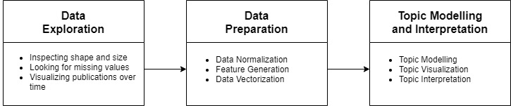
Data Exploration

The first part of the topic extraction process is concerned with the exploration of the structure and content of the dataset. This includes a first view of the raw data, checks on missing values, and the visualization of publications on a time axis to reveal underlying trends.

Dataset Structure

We start by importing Pandas and loading a single entry of the dataset into a DataFrame. Printing the content for visual inspection reveals that the raw data consists of fourteen distinct columns. The next step is then to filter the dataset to only retain data necessary for trend detection and topic modeling. Therefore we only include the title, abstract, category, and publication date of the papers.

After settling on the required information, all records of the aforementioned four columns are imported and converted into a DataFrame. A quick check for possible missing values in the data reveals a well-maintained dataset without missing entries. The shape of the DataFrame is set at around 1.9 million entries with four columns.

Visualizing Publication Trends

From here we leverage the categories of the papers to visualize the number of publications per scientific field over time. This should determine the direction for further analysis and reduce the ambiguity of the relatively large dataset. We create a first view of the dataset by counting the publications per category:

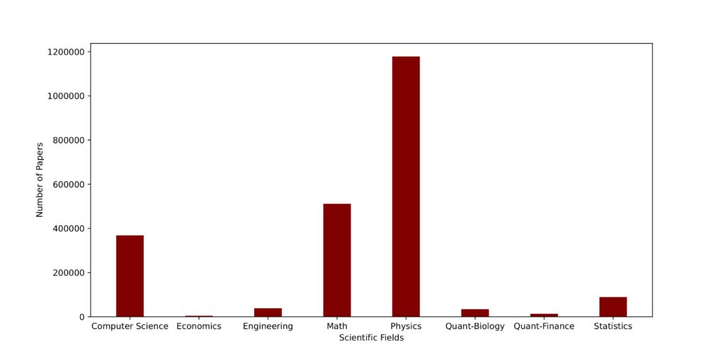
As can be seen in the bar graph, the vast majority of publications are contained in the physics group with math in second and computer science in third place. Given that a scientific paper can have more than one category, the bar graph counts more publications than contained in the initial dataset. Nonetheless, for a general overview, this is sufficient.

To detect trends, the next step is to display the publications as a time series. We split the publications by category and group them by their publication date. For better visibility and to smooth the trendline, we also compute a 3-month moving average of the publications. Additionally, we restrict the graph to publications after the year 1999.

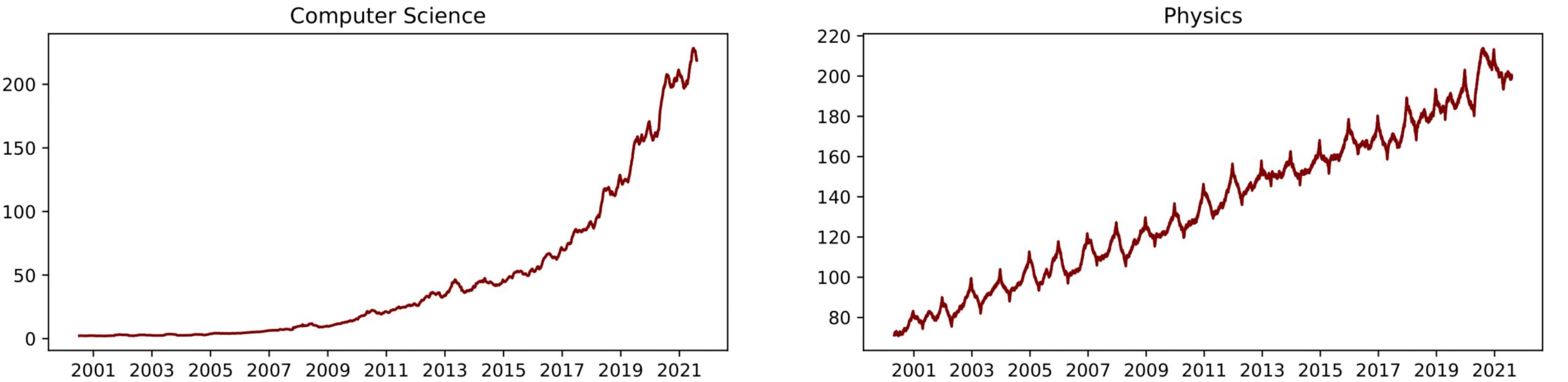
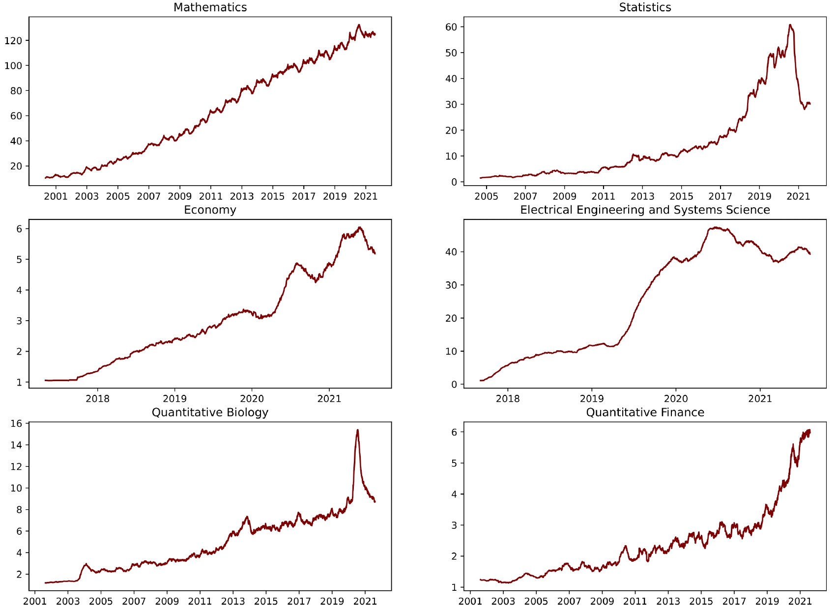
Looking at the trendlines, we can see that scientific publications, in general, are on an upwards trend. Nonetheless, if the timeframe is restricted to the most recent years, computer science and physics can be considered the top trending fields if we lay our focus solely on the number of published papers. The publication frequency at the moment is thereby around an average of two hundred publications per day, with an upwards tendency. From here on we will restrict the dataset to these two categories and to publications made after the year 2019, to get the most current topics.

Data Preparation

After settling on our two major scientific fields, we will now prepare the text data for topic modeling. This step includes first of all splitting the data into two separated DataFrames (one for each field), the generation of new features from the existing data, and following the vectorization of the text corpus to make the data suitable for downstream algorithms.

Feature Generation and Vectorization

To facilitate the interpretability of the extracted topics, we extract the nouns of the respective abstracts. Nouns are more suitable for general topic modeling because nouns carry the most meaning inside a text. This step also reduces the amount of text data to be analyzed and speeds up the topic modeling process. To further clean the data, extracted nouns containing special characters are removed and all text is set to lowercase.

Following we use the TF-IDF method to vectorize the extracted nouns. This step gets us two sparse matrices which we can now use for topic modeling. Additionally, we also have a list of feature names that we will use for topic visualization.

Topic Modeling

After completion of the data preparation step, we can now feed the TF-IDF matrix into our topic modeling algorithm (LDA). Given that the number of topics must be set before generating a topic, this step usually involves a lot of trial and error. After testing different parameters, the generation of twenty topics from each of the two categories subjectively leads to the best interpretability of the resulting topics.

Interpretation

To facilitate the interpretation of the generated topics, we will leverage the sub-categories of the publications that were part of the dataset. Given that the sub-categories with the most publications can also be considered to be the most trending categories, a word cloud is a quick and easy method to extract the top categories from the two DataFrames. The word cloud on the left represents computer science and the word cloud on the right physics:

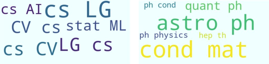
With the help of the category taxonomy published on the arXiv website, the category tags can be interpreted. Thereby the most frequently occurring categories for computer science are machine learning (cs.LG, stat.ML), artificial intelligence (cs.AI) and computer vision (cs.CV). For physics, the categories astrophysics (astro-ph), condensed matter (cond-mat), and quantum
physics (quant-ph) are the top trending categories. A full list of categories can be viewed on the arXiv website.

To finally determine the trending topics in detail, we look at what topics were generated by the LDA algorithm. To make interpretation more feasible, we display the five most frequent words of a specific topic as a vertical bar graph. Here is an example from computer science and physics respectively:

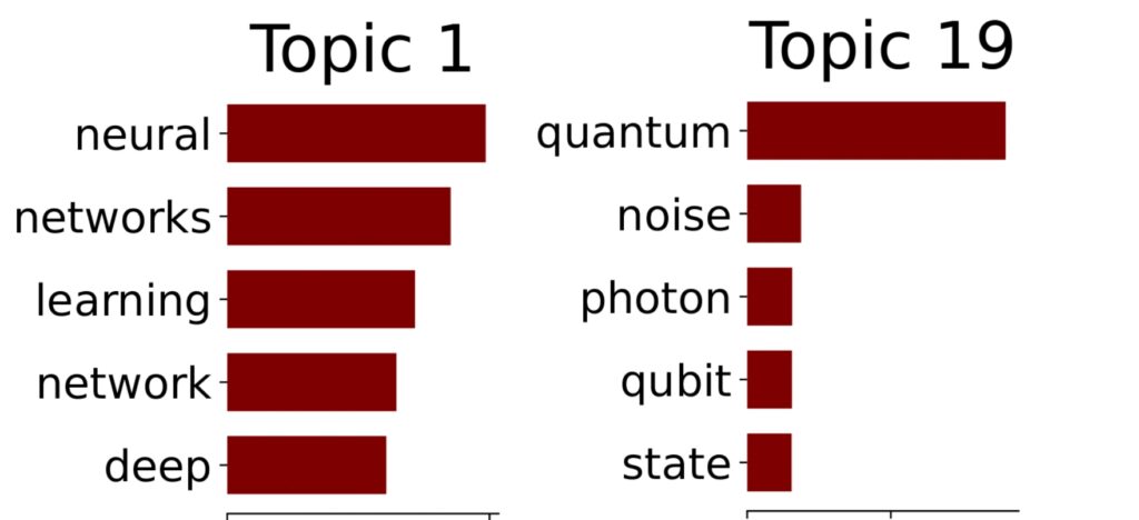
A possible interpretation would be that topic 1 from computer science can be interpreted to be centered around neural networks and deep learning and topic 19 from physics concerning itself with quantum computing. The full list of generated topics can be viewed here for computer science and here for physics.

Detecting Trends

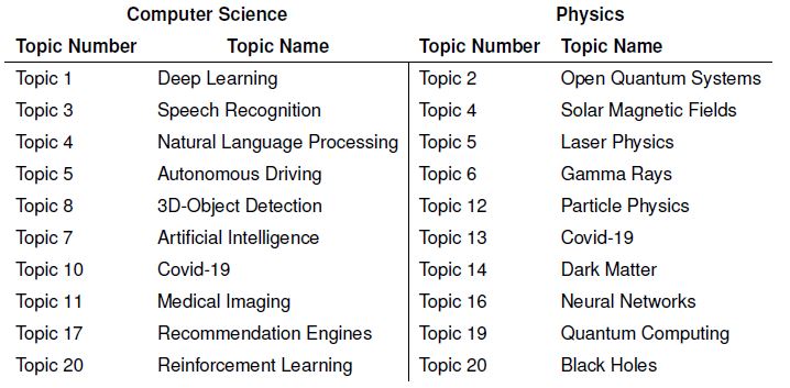
Given the results of our preceding analysis of the arXiv dataset, we can detect a lot of possible trends in current research. Focusing on the two major categories computer science and physics and further with the most common sub-categories in mind, the following table shows topics that I could derive from the results:

Conclusion

Identifying trends in science is valuable for a lot of reasons. Funding can be strategically allocated to efficiently support current trends and research cooperations can be established in fields that have a lot of traction. This offers a mutual benefit to both researchers and the supporting stakeholders. The code for the analysis can be found in this GitHub repo.

References

Bengfort, B., Bilbro, R., & Ojeda, T. (2018). Applied text analysis with python: Enabling language aware data products with machine learning. Sebastopol, CA: O’Reilly Media.
Berry, M. W. (Ed.). (2004). Survey of text mining: Clustering, classification, and retrieval. New York, NY: Springer.
Bird, S., Klein, E., & Loper, E. (2009). Natural language processing with python. Sebastopol: O’Reilly Media Inc.
Blei, D. M., Ng, A. Y., & Jordan, M. I. (2003). Latent dirichlet allocation. the Journal of machine Learning research(3), 993–1022.
Cornell University. (2021). Category taxonomy. Retrieved from https://arxiv.org/category_taxonomy
Cutting, D., Kupiec, J., Pedersen, J., & Sibun, P. (1992). A practical part-of-speech tagger. Proceesings of the third conference on applied natural language processing, 133.
Fiona Martin, & Mark Johnson. (2015). More efficient topic modelling through a noun only approach. In Alta.
Lane, H., Howard, C., & Hapke, H. (2019). Natural language processing in action: Understanding, analyzing, and generating text with python. Shelter Island: Manning.
Petrov, S., Das, D., & McDonald, R. (2011). A universal part-of-speech tagset. Computing Research Repository.
Prabhakaran, V., Hamilton, W. L., McFarland, D., & Jurafsky, D. (2016). Predicting the rise and fall of scientific topics from trends in their rhetorical framing. Proceedings of the 54th annual meeting of the association for computational linguistics.
Roy, S., Gevry, D., & Pottenger, W. (2002). Methodologies for trend detection in textual data mining.
Schachter, P., & Shopen, T. (2007). Parts-of-speech systems. Language typology and syntactic description, 1–60.
Voutilainen, A. (2012). Part-of-speech tagging. The Oxford Handbook of Computational Linguistics.
Witten, I. H., Pal, C. J., Frank, E., & Hall, M. A. (2017). Data mining: Practical machine learning tools and techniques (4th ed.). Cambridge, MA: Morgan Kaufmann.