Why Are Financial Time Series Called Random Walks?

Financial time series are notoriously hard to model and are often referred to as random walks. But why? In this article, we will take a closer look at what a random walk is and the reasons why financial time series are described as such. As a prerequisite for a full comprehension of the article, a basic understanding of general time series analysis and ARMA models is necessary.

What is a financial time series?

A financial time series is a type of data that chronicles the evolution of prices or other relevant economic indicators over certain periods of time. A series typically contains information on currency exchange rates, stock prices, or market indices. Financial time series analysis is the process of studying such time series to identify patterns and trends that could be useful for forecasting. As an example of a financial time series, the graph below shows daily Bitcoin closing prices for the year 2021.

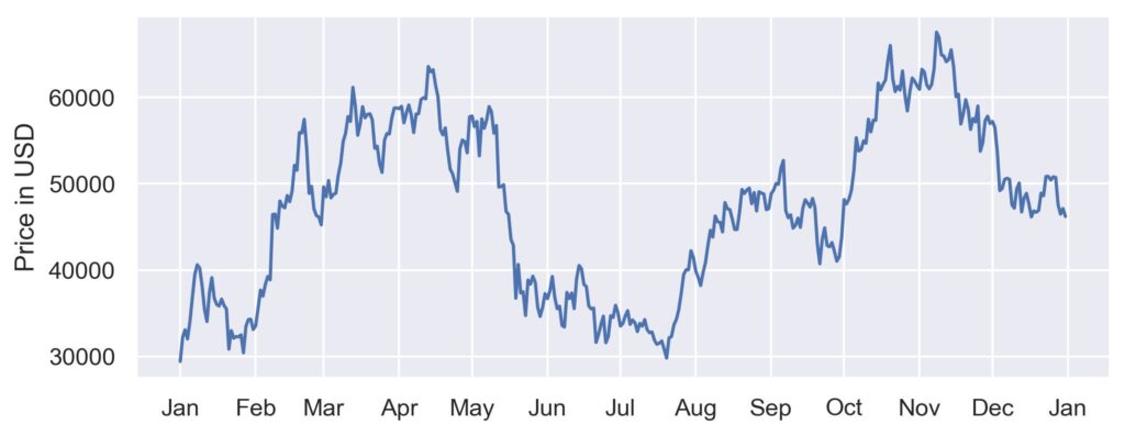
One of the main difficulties when modeling financial time series is that the data tends to be non-stationary, which means that the mean and variance of the data change over time. This makes it difficult to make accurate predictions, as different models may apply at different points in time. Furthermore, financial markets are highly volatile and subject to rapid change due to external factors such as news reports and political events. This makes it hard to accurately predict future movements in prices using historical information alone, since current trends may not remain consistent over a long period of time.

Modeling techniques

There are various methods for modeling general time series, for example, linear regression, moving averages, Holt-Winters, and ARMA models, though not all of these models work well for financial time series. The focus of this article will be on ARMA models, and for now, let us examine the basics and tackle the problem of the non-stationarity of financial time series. The basic ARMA models need at least the assumption of weak stationarity to work properly, which means we have a constant mean, finite variance, and the covariance between two observations depends only on the distance between them. To recall, the classic ARMA model consists of the autoregressive (AR) and the moving average (MA) model. A method for achieving stationarity is differencing where we subtract a lagged version of the time series from itself. So let us look at the following plot.

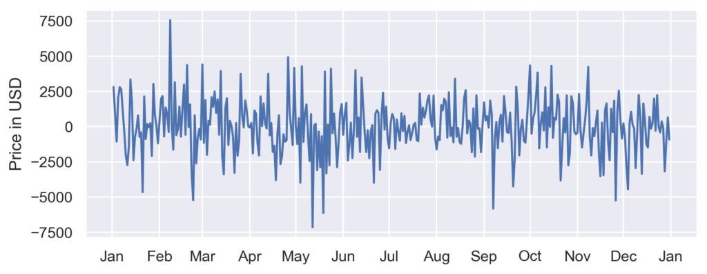
The plot shows again the Bitcoin closing prices but this time the values at the first lag t-1 were subtracted from the value at time t. We can see that the differences in price look like they have no visible trend, which means we should have achieved stationarity. But how can we be (a bit more) certain?

Testing for stationarity

To aid the visual inspection, there are statistical tests for addressing the stationarity concern, with one of these tests being the Dickey-Fuller (DF) test and its expanded version, the Augmented-Dickey-Fuller (ADF) test. The DF test works by examining if we have a unit-root process. So given the AR(1) model denoted by $X_{t} =\phi X_{t-1} + \epsilon_{t}$ we have a unit root process if $\phi=1$. Therefore, the DF test has the following hypotheses:
$$ \begin{aligned} & H_0: \phi=1\\ & H_1:|\phi|<1 & \end{aligned} $$ The problem is that the DF test is only meaningful if we can model our time series with an AR(1) model. To account for this shortcoming, the ADF test was created which can be used for all ARMA(p,q) models. Now let us examine the following ACF and PACF plots of the BTC closing prices:

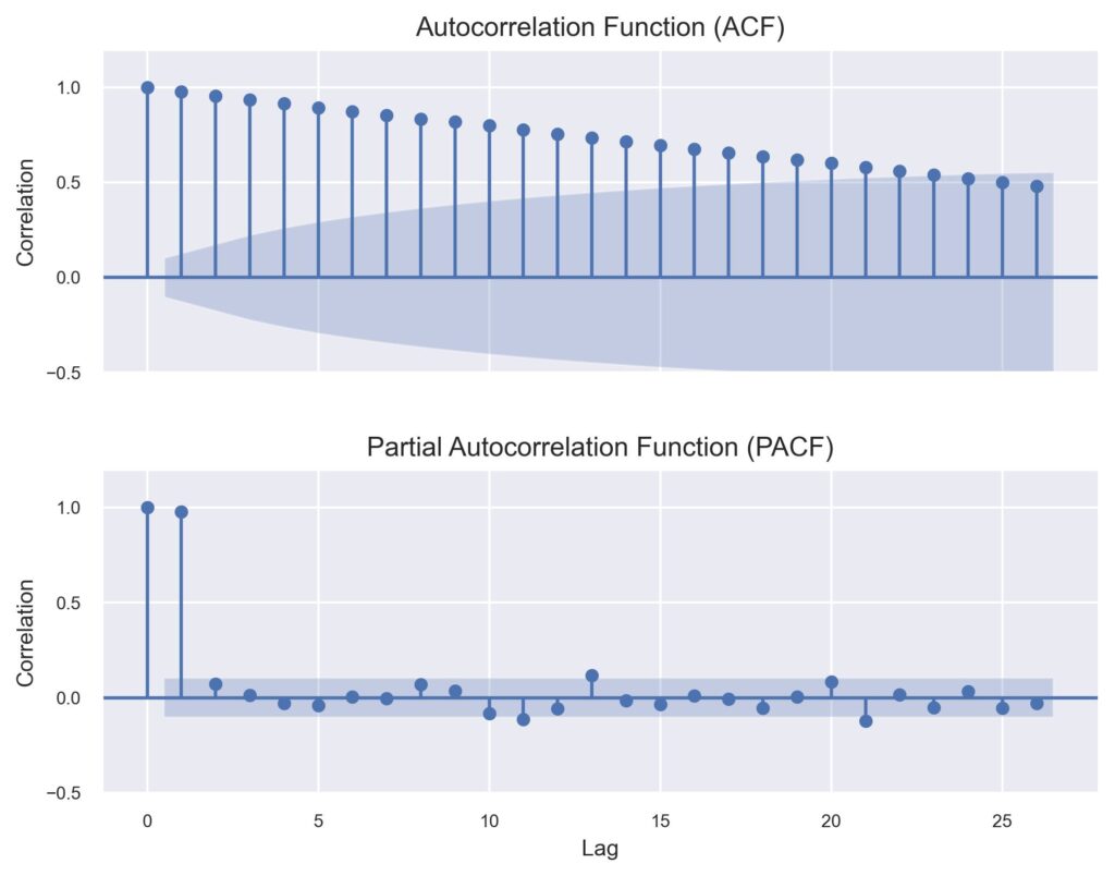
Although the PACF plot cuts off after the first lag, which would be suitable for an AR(1) model, the ACF is only slowly tailing off instead of the exponential decrease that we would like to see. This means two things, first the AR(1) is not a suitable model, and second, we have our first bit of evidence for a unit root in our time series because this ACF pattern is common for unit root processes.  Applying the ADF test yields around -2.34 for the ADF test statistic and a p-value of 0.158 which means we cannot reject our null hypothesis of having a unit root. In contrast, if we apply the ADF test to the differenced time series we get an ADF test statistic of around -20.1 and an extremely small p-value which lets us reject the null hypothesis and accept that the differenced series is stationary. So now we can start fitting an ARMA model, or?

Random walks

A random walk is a process in probability theory where the probable location of a point is determined based on random motions, with probabilities of moving some distance in some direction being the same at each step. To illustrate this we plot the correlogram of the differenced closing prices.

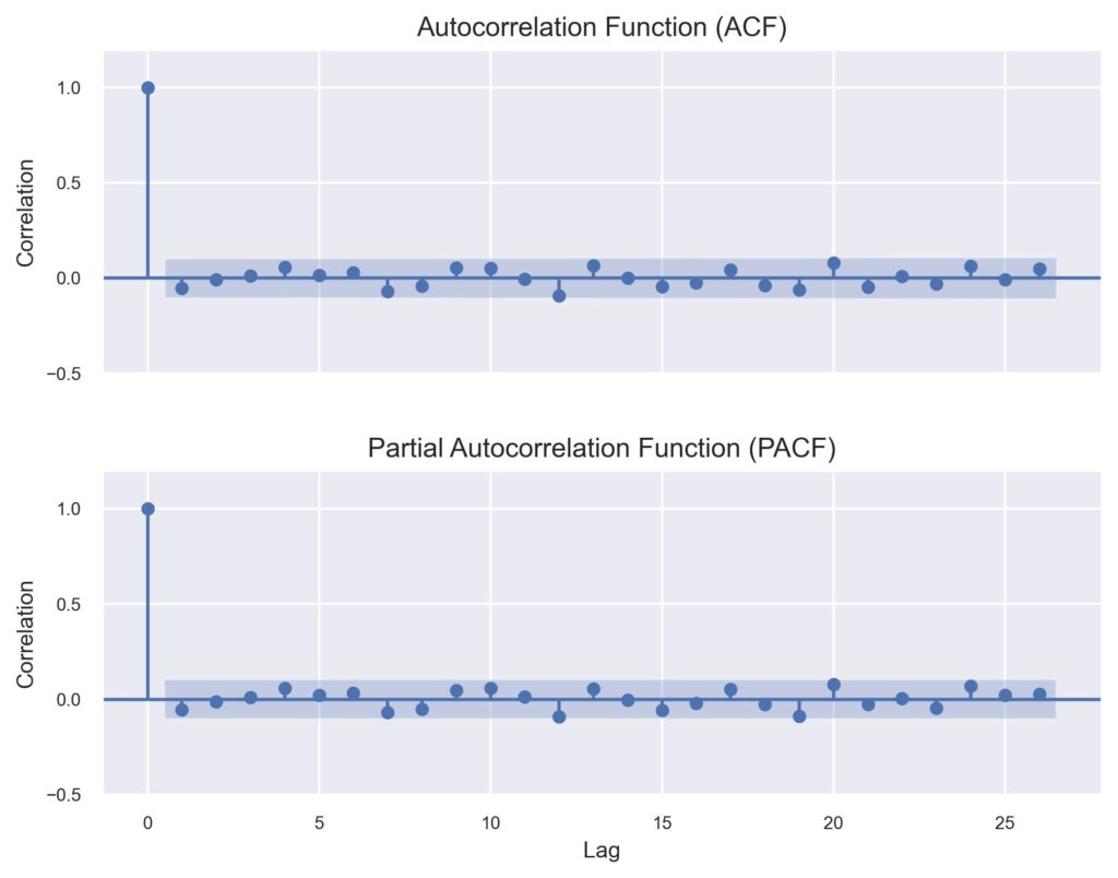
This plot of the ACF and PACF of the differenced series sums up why financial time series are described as random walks. As we can see there is no autocorrelation to be found and the only model we can fit would be an ARMA(0,0) which, let’s be real, would not be of particular help for making money in the stock market.

Conclusion

In this article, we looked into the basics of financial time series and modeling techniques, focusing on ARMA models and their prerequisites. Additionally, we spoke about the concept of stationarity and how to objectively assess it. Finally, we discussed random walks and showed why financial time series are called random walks by analyzing the correlogram of a stationary series of differenced daily BTC closing prices. We conclude with the finding that future prices can not be predicted by past prices, at least not with classical ARMA models.

References

Adrian, T. (2022). Interest Rate Increases, Volatile Markets, Signal Rising Financial Stability Risks. Retrieved from https://www.imf.org/en/Blogs/Articles/2022/10/11/interest-rate-increases-volatile-markets-signal-rising-financial-stability-risks
Encyclopedia Britannica (2023). Random walk. Retrieved from https://www.britannica.com/science/random-walk
Iordanova, T. (2022). An Introduction to Non-Stationary Processes. Investopedia. Retrieved from https://www.investopedia.com/articles/trading/07/stationary.asp
Montgomery, D. C., Jennings, C. L., & Kulahci, M. (2008). Introduction to time series analysis and forecasting. Wiley series in probability and statistics. Hoboken, NJ: Wiley
Shumway, R. H., & Stoffer, D. S. (2006). Time Series Analysis and Its Applications: With R Examples (2nd ed.). SpringerLink Bücher. Cham: Springer
Tsay, R. S. (2005). Analysis of financial time series (2nd ed.). Wiley series in probability and statistics. Hoboken, NJ: Wiley
Zivot, E., & Wang, J. (2006). Modeling Financial Time Series with S-PLUS® (2nd ed.). New York, NY: Springer New York